Fit a straight line y = ax+b and also parabola y = ax^2+bx+c . Also calculate Sum of Residuals in each case.
Introduction:
The least squares approach is a vital tool in the fields of data analysis and curve fitting. It allows us to determine which line or curve, given a series of data points, best fits the data. This article explores how to fit straight lines and parabolas to data sets using the least squares method. We will examine the fitting procedure, the mathematical formulas, and the computation of the total residuals for every example.
Fitting a Straight Line (y = ax + b):
A straight line’s equation is written as y = ax + b, where a is the slope and b is the y-intercept. The goal of the least squares approach is to reduce the sum of squared disparities between the actual and expected values of y for every x.
Let’s take a mathematical example where we have n data points (x i, y i ) where p = 1, 2,… and i = 1, 2,…, n. Finding the values of A and B that minimize the sum of squared residuals, or S, is our goal:
S = ∑ ni = 1 (y i −(ax i + b))2
We differentiate 𝑆 with respect to 𝑎 and 𝑏, set the derivatives to zero, then solve the ensuing system of equations to determine the ideal values of 𝑎 and 𝑏. We can plot the straight line that best matches the data points after we know a and b. In addition, the derived values of a and b can be substituted back into the equation for S to get the total of residuals.
Fitting a Parabola (y = ax² + bx + c):
The equation y =ax2+bx+c, where a determines the curvature, b shifts the vertex along the x-axis, and c shifts it along the y-axis, represents a parabola. We aim to minimize the sum of squared differences between the observed and anticipated values of y, just like when fitting a straight line.
The goal is to determine the values of A, B, and C that minimize the sum of squared residuals, or S, given the same set of data points (x i, y i):
𝑆= ∑n𝑖= 1 (𝑦𝑖−(𝑎𝑥𝑖2) + 𝑏𝑥𝑖 +𝑐))2
Using a similar method to the straight line case, we determine the ideal values of a, b, and c.
After setting the derivatives to zero and differentiating 𝑆 S with respect to each parameter, we solve the ensuing system of equations. The normal equations are a system of linear equations that are produced by the use of partial derivatives and matrix calculations.
Finding the coefficients a, b, and c allows us to plot the parabolic curve that most closely matches the data points. Similar calculations can be made for the sum of residuals by returning the obtained values for a, b, and c to the equation for 𝑆.
Sum of Residuals:
The entire difference between the observed and expected values of y is represented by the sum of residuals. For both straight line and parabola fitting, a lower total of residuals signifies a more favorable fit to the data.
We may evaluate the correctness of our fitted model by computing the sum of the residuals. A close to zero sum of residuals indicates that our model successfully reflects the underlying trend in the data. A significant sum of residuals, on the other hand, suggests that the model might not fully capture the data points, which calls for a review of the fitting procedure.
Conclusion:
A useful technique for fitting mathematical models to data sets is the least squares method. The goal is always the same when fitting a parabola or a straight line: to reduce the sum of squared discrepancies between the values that are seen and those that are anticipated. The best-fitting model’s ideal parameters can be found by applying mathematical methods like differentiation and system of equations solutions.
Comprehending the ideas and computations associated with fitting parabolas and straight lines improves our capacity to evaluate information and arrive at wise conclusions. Furthermore, the analysis of the sum of residuals offers important information on the precision and dependability of our fitted models. We get a greater understanding of the least squares method as we investigate and use it in more fields.
Question:
Fit a straight line y = ax + b and also a parabola y = ax^2 +bx +c to the following set of observations. Also calculate sum of squares of the residuals in each case and test which curve is more suitable to the data.
|
x |
0 |
1 |
2 |
3 |
4 |
|
y |
1 |
5 |
10 |
22 |
38 |
Fit a straight line y = ax + b and also a parabola y = ax^2 +bx +c to the following set of observations. Also calculate sum of squares of the residuals in each case and test which curve is more suitable to the data.
|
x |
0 |
1 |
2 |
3 |
4 |
|
y |
1 |
5 |
10 |
22 |
38 |
Solution:
Let
y = ax + b…………………(A) ( Fitting a straight line)
Normal equations are :
∑ y = a∑x +nb…………………………..(1)
∑ x y = a∑ + b∑x………………………(2)

from (1 )
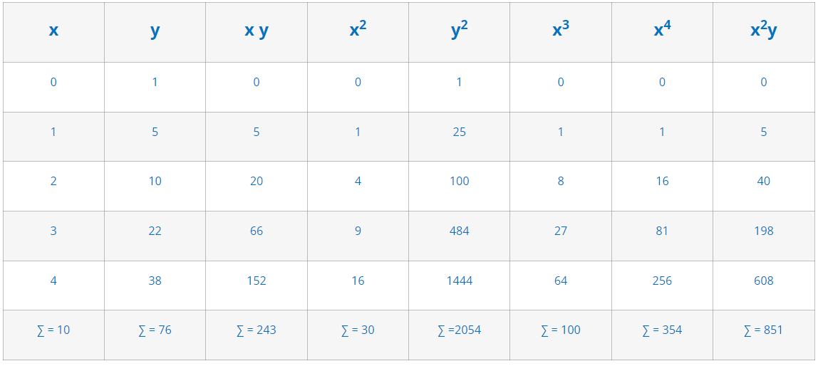
76 = 10a+ 5b…………………(3)
From( 2)
243 = 30a +10b……………….(4)
Eq( 4 )– 3 eq( 1)
243 = 30a +10b
228 = 30a +15b
15 = – 5b
b = – 3
put in( 3)
76 = 10a + 5( -3)
a = 9.1
put in eq (A)
y = 9.1 x – 3
let E1 be sum of squares of residuals:
E1 = ∑y2 – a ∑xy – b ∑y
= 2054 – 243 (9.1) – 76 ( -3 )
E1 = 70.7
2) y = ax2 + bx + c…………………(B) (fitting a parabola)
Normal equations are :
∑y = a∑ + b∑x + nc…………………(1)
∑xy = a∑ + b∑ + c∑x……………(2)
∑y = a∑ + b∑ + c∑………(3)
From (1)
76 = 30a+ 10b +5c………………………………….(4)
From (2)
243 = 100a +30b+ 10c………………………………(5)
From (3)
851 = 354a +100b+ 30c……………………………..(6)
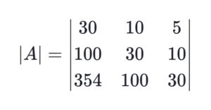
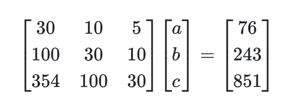
Using Cramer’s Rule:
A X = B 

= 30 – 10 + 5
= 30 900 – 1000 – 10 3000 – 3540 + 5 10000 – 10620
|A| = – 700

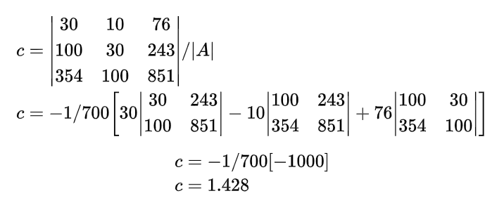
= – 1 / 700 [ 76 – 10 + 5 ]
a = – 1 / 700 [ – 1550 ]
a = 2.214
Similarly,

= – 1 / 700 [ 30 – 76 + 5 ]
= – 1 / 700 [ – 170 ]
b = 0.292
Now,

Put in eq B
y = ax2 + bx
y = 2.2 + 0.3b + 1.4
Let be the sum of squares of residuals:
E2 = ∑y2 – a ∑x2y – b ∑ xy – c ∑ y
= 2054 – 851 (2.214) – 243 ( 0.242)– 76 (1.428)
E2 = 2.55
Since,
E2 < E1 So clearly the parabola is better fit than the straight line.
Frequently Asked Questions (FAQs)
Q) What is the least square method?
A mathematical method called the least squares method can be used to determine which curve best fits a given set of data points. It reduces the total squared discrepancies between the values that were seen and those that were projected.
Q) How does the least square method work?
The least squares approach minimizes the sum of squared residuals by identifying the parameters of a mathematical model. Usually, to do this, the derivatives are set to zero and the sum of squared residuals are differentiated with respect to the parameters.
Q) What is the significance of the least square method?
Numerous disciplines, including statistics, engineering, physics, and economics, frequently employ the least squares approach. It offers a methodical approach to fitting mathematical models to data, empowering researchers to forecast and derive inferences from empirical data
Q) How is the sum of residuals calculated?
The difference, squared, between the observed and anticipated values of the dependent variable (y) for each data point is the sum of residuals. The entire difference between the data and the fitted model is represented by this sum.
Q) Can the least square method fit any type of curve?
The efficiency of the least squares method is dependent on the intricacy of the curve and the quality of the data, despite its versatility and ability to fit a wide range of curves. Alternative fitting techniques could be needed for curves that are more complicated, including nonlinear functions or higher-order polynomials.
Q) What is the difference between fitting a straight line and a parabola using the least square method?
The slope and intercept that minimize the sum of squared discrepancies between the observed and anticipated y-values are needed to fit a straight line. The coefficients of the quadratic equation that minimize the sum of squared residuals must be found in order to fit a parabola. In the latter case, a system of linear equations that are based on partial derivatives must be solved.
Q) How do you assess the quality of a fitted model using the sum of residuals?
A better match between the model and the data is indicated by a smaller total of residuals. It is imperative to take into account additional variables, such as the intricacy of the model and the problem’s context. Visual examination of the fitted curve in relation to the data points may also be required in specific circumstances.
Q) Are there limitations to the least square method?
The least squares approach has drawbacks while being popular and useful for a variety of applications. For example, it makes the assumption that the data’s flaws are independent and regularly distributed. Furthermore, it could not function effectively in data sets with a lot of unpredictability or outliers. Alternative approaches or data preprocessing strategies might be required in these circumstances.

